Quickstart + Usage
After installing Consenrich, run it from the command line with
consenrich -h or import it from Python.
The examples below are intentionally short demos on a couple chromosomes.
Getting Started: H3K27ac ChIP-seq
This minimal example estimates a consensus H3K27ac signal from four ENCODE epidermis ChIP-seq experiments with matched input controls.
Input Data
Experiment |
Biosample |
H3K27ac alignment |
Control alignment |
|---|---|---|---|
Epidermis/Female/71 |
|||
Epidermis/Male/67 |
|||
Epidermis/Female/80 |
|||
Epidermis/Male/75 |
Download Alignments
Copy and paste the following into your terminal to download and index the BAM
files. You can use curl -L -O <URL> in place of wget <URL> if wget
is not available.
encodeFiles=https://www.encodeproject.org/files
for file in ENCFF793ZHL ENCFF647VPO ENCFF809VKT ENCFF295EFL; do
    wget "$encodeFiles/$file/@@download/$file.bam"
done
for ctrl in ENCFF444WVG ENCFF619NYP ENCFF898LKJ ENCFF490MWV; do
    wget "$encodeFiles/$ctrl/@@download/$ctrl.bam"
done
samtools index -M *.bam
YAML Configuration
Save the following as demoHistoneChIPSeq.yaml in the directory containing
the BAM files:
experimentName: demoHistoneChIPSeq

genomeParams:
  name: hg38
  chromosomes: [chr21, chr22]
  excludeForNorm: [chrX, chrY]

inputParams:
  samples:
    - name: H3K27ac_1
      path: ENCFF793ZHL.bam
      format: bam
      role: treatment
    - name: H3K27ac_2
      path: ENCFF647VPO.bam
      format: bam
      role: treatment
    - name: H3K27ac_3
      path: ENCFF809VKT.bam
      format: bam
      role: treatment
    - name: H3K27ac_4
      path: ENCFF295EFL.bam
      format: bam
      role: treatment
    - name: input_1
      path: ENCFF444WVG.bam
      format: bam
      role: control
    - name: input_2
      path: ENCFF619NYP.bam
      format: bam
      role: control
    - name: input_3
      path: ENCFF898LKJ.bam
      format: bam
      role: control
    - name: input_4
      path: ENCFF490MWV.bam
      format: bam
      role: control
Run Consenrich
% consenrich --config demoHistoneChIPSeq.yaml --verbose
The run writes a state bedGraph, uncertainty bedGraph, state bigWig, uncertainty bigWig, ROCCO narrowPeak file, and ROCCO gappedPeak file. With the current package version, the principal output files are:
demoHistoneChIPSeq_consenrich_state.VERSION.bw
demoHistoneChIPSeq_consenrich_uncertainty.VERSION.bw
consenrichOutput_demoHistoneChIPSeq_state.VERSION_rocco.narrowPeak
consenrichOutput_demoHistoneChIPSeq_state.VERSION_rocco.gappedPeak
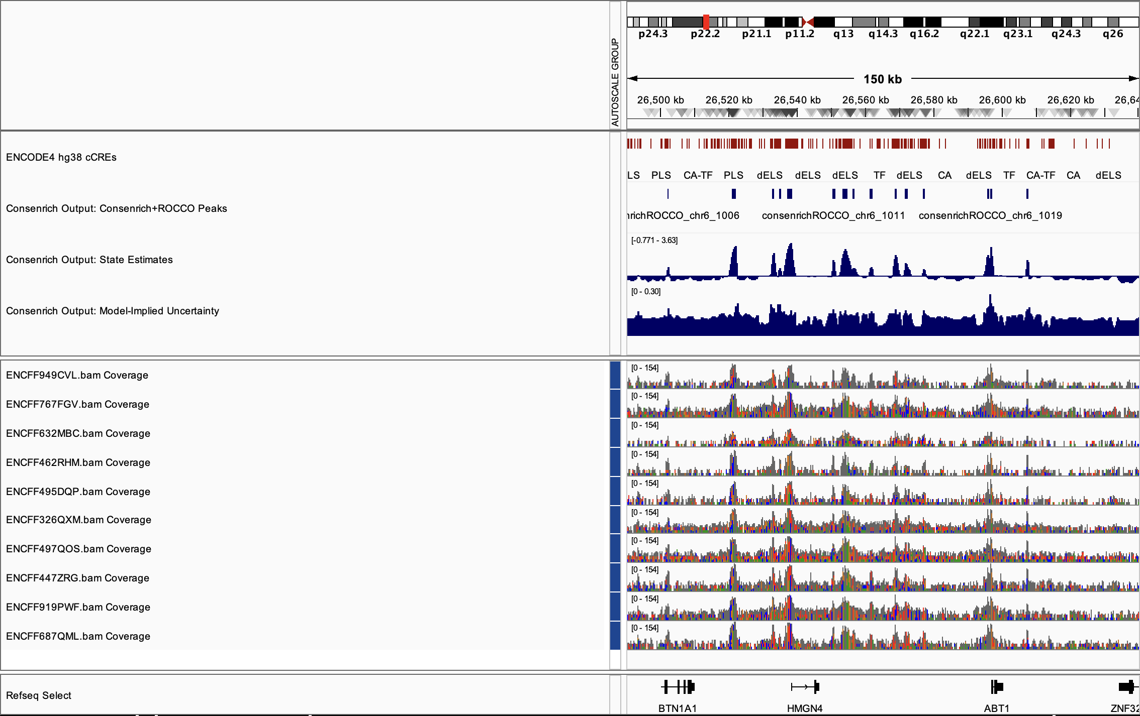
ATAC-seq Demo
This demo estimates a consensus chromatin-accessibility signal from ten ENCODE ATAC-seq alignments.
Download Alignments
encodeFiles=https://www.encodeproject.org/files
for file in ENCFF326QXM ENCFF447ZRG ENCFF462RHM ENCFF495DQP ENCFF497QOS ENCFF632MBC ENCFF687QML ENCFF767FGV ENCFF919PWF ENCFF949CVL; do
    wget "$encodeFiles/$file/@@download/$file.bam"
done
samtools index -M *.bam
YAML Configuration
Save the following as atacDemo.yaml:
experimentName: atacDemo

genomeParams:
  name: hg38
  # chromosomes: [chr11, chr22] # faster: Uncomment and specify chromosomes
  excludeForNorm: [chrX, chrY]

inputParams:
  bamFiles:
    - ENCFF326QXM.bam
    - ENCFF447ZRG.bam
    - ENCFF462RHM.bam
    - ENCFF495DQP.bam
    - ENCFF497QOS.bam
    - ENCFF632MBC.bam
    - ENCFF687QML.bam
    - ENCFF767FGV.bam
    - ENCFF919PWF.bam
    - ENCFF949CVL.bam
Run Consenrich
% consenrich --config atacDemo.yaml --verbose
Principal output files:
atacDemo_consenrich_state.VERSION..bw
atacDemo_consenrich_uncertainty.VERSION.bw
consenrichOutput_atacDemo_state.VERSION_rocco.narrowPeak
consenrichOutput_atacDemo_state.VERSION_rocco.gappedPeak
Results
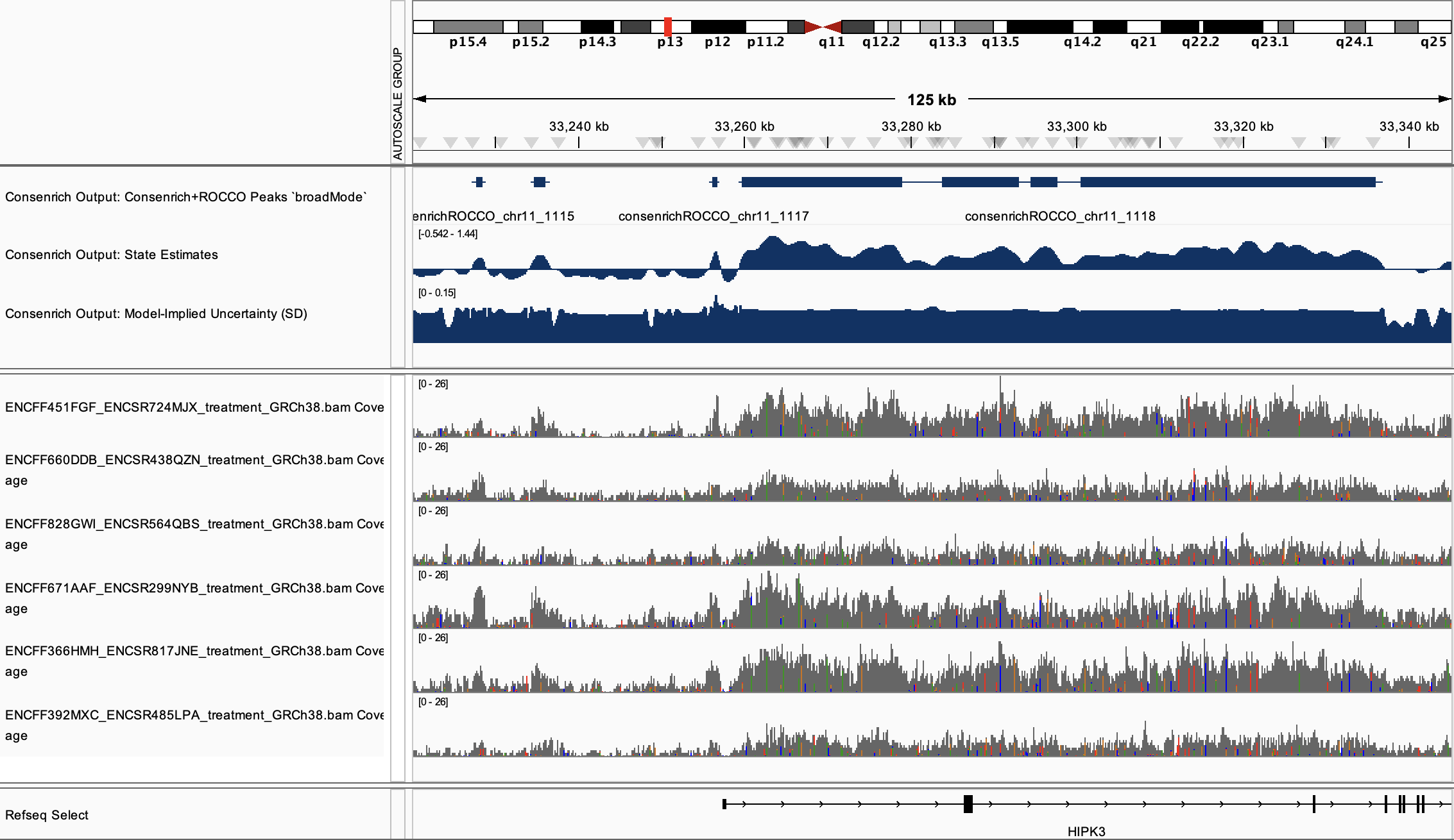
Broad Mark ChIP-seq Demo
Download Alignments
(This will take a while!)
encodeFiles=https://www.encodeproject.org/files

while read -r accession output; do
    wget -O "$output" "$encodeFiles/$accession/@@download/$accession.bam"
done <<'EOF'
ENCFF365LTV ENCFF365LTV_ENCSR449FRQ_treatment_GRCh38.bam
ENCFF630KZV ENCFF630KZV_ENCSR678RFS_treatment_GRCh38.bam
ENCFF851FLQ ENCFF851FLQ_ENCSR412THE_treatment_GRCh38.bam
ENCFF581VRR ENCFF581VRR_ENCSR208XKJ_treatment_GRCh38.bam
ENCFF451FGF ENCFF451FGF_ENCSR724MJX_treatment_GRCh38.bam
ENCFF660DDB ENCFF660DDB_ENCSR438QZN_treatment_GRCh38.bam
ENCFF828GWI ENCFF828GWI_ENCSR564QBS_treatment_GRCh38.bam
ENCFF392MXC ENCFF392MXC_ENCSR485LPA_treatment_GRCh38.bam
ENCFF366HMH ENCFF366HMH_ENCSR817JNE_treatment_GRCh38.bam
ENCFF671AAF ENCFF671AAF_ENCSR299NYB_treatment_GRCh38.bam
ENCFF536MLZ ENCFF536MLZ_ENCSR178FVP_control_GRCh38.bam
ENCFF007LNN ENCFF007LNN_ENCSR632MPN_control_GRCh38.bam
ENCFF422MKH ENCFF422MKH_ENCSR040TRJ_control_GRCh38.bam
ENCFF525NLT ENCFF525NLT_ENCSR979YKY_control_GRCh38.bam
ENCFF013ION ENCFF013ION_ENCSR109IWL_control_GRCh38.bam
ENCFF730PAF ENCFF730PAF_ENCSR526EXI_control_GRCh38.bam
ENCFF971XWL ENCFF971XWL_ENCSR945LPX_control_GRCh38.bam
ENCFF273EYI ENCFF273EYI_ENCSR120ITZ_control_GRCh38.bam
ENCFF944AYC ENCFF944AYC_ENCSR061EXX_control_GRCh38.bam
ENCFF271VZL ENCFF271VZL_ENCSR261PLD_control_GRCh38.bam
EOF

samtools index -M *.bam
YAML Configuration
Save the following as bigH3K4me1Demo.yaml:
experimentName: bigH3K4me1Demo

genomeParams:
  name: hg38
  chromosomes: [chr21, chr22]
  excludeForNorm: [chrX, chrY]

inputParams:
  samples:
    - name: ENCSR449FRQ_H3K4me1
      path: ENCFF365LTV_ENCSR449FRQ_treatment_GRCh38.bam
      format: bam
      role: treatment
    - name: ENCSR678RFS_H3K4me1
      path: ENCFF630KZV_ENCSR678RFS_treatment_GRCh38.bam
      format: bam
      role: treatment
    - name: ENCSR412THE_H3K4me1
      path: ENCFF851FLQ_ENCSR412THE_treatment_GRCh38.bam
      format: bam
      role: treatment
    - name: ENCSR208XKJ_H3K4me1
      path: ENCFF581VRR_ENCSR208XKJ_treatment_GRCh38.bam
      format: bam
      role: treatment
    - name: ENCSR724MJX_H3K4me1
      path: ENCFF451FGF_ENCSR724MJX_treatment_GRCh38.bam
      format: bam
      role: treatment
    - name: ENCSR438QZN_H3K4me1
      path: ENCFF660DDB_ENCSR438QZN_treatment_GRCh38.bam
      format: bam
      role: treatment
    - name: ENCSR564QBS_H3K4me1
      path: ENCFF828GWI_ENCSR564QBS_treatment_GRCh38.bam
      format: bam
      role: treatment
    - name: ENCSR485LPA_H3K4me1
      path: ENCFF392MXC_ENCSR485LPA_treatment_GRCh38.bam
      format: bam
      role: treatment
    - name: ENCSR817JNE_H3K4me1
      path: ENCFF366HMH_ENCSR817JNE_treatment_GRCh38.bam
      format: bam
      role: treatment
    - name: ENCSR299NYB_H3K4me1
      path: ENCFF671AAF_ENCSR299NYB_treatment_GRCh38.bam
      format: bam
      role: treatment

    - name: ENCSR178FVP_input_for_ENCSR449FRQ
      path: ENCFF536MLZ_ENCSR178FVP_control_GRCh38.bam
      format: bam
      role: control
    - name: ENCSR632MPN_input_for_ENCSR678RFS
      path: ENCFF007LNN_ENCSR632MPN_control_GRCh38.bam
      format: bam
      role: control
    - name: ENCSR040TRJ_input_for_ENCSR412THE
      path: ENCFF422MKH_ENCSR040TRJ_control_GRCh38.bam
      format: bam
      role: control
    - name: ENCSR979YKY_input_for_ENCSR208XKJ
      path: ENCFF525NLT_ENCSR979YKY_control_GRCh38.bam
      format: bam
      role: control
    - name: ENCSR109IWL_input_for_ENCSR724MJX
      path: ENCFF013ION_ENCSR109IWL_control_GRCh38.bam
      format: bam
      role: control
    - name: ENCSR526EXI_input_for_ENCSR438QZN
      path: ENCFF730PAF_ENCSR526EXI_control_GRCh38.bam
      format: bam
      role: control
    - name: ENCSR945LPX_input_for_ENCSR564QBS
      path: ENCFF971XWL_ENCSR945LPX_control_GRCh38.bam
      format: bam
      role: control
    - name: ENCSR120ITZ_input_for_ENCSR485LPA
      path: ENCFF273EYI_ENCSR120ITZ_control_GRCh38.bam
      format: bam
      role: control
    - name: ENCSR061EXX_input_for_ENCSR817JNE
      path: ENCFF944AYC_ENCSR061EXX_control_GRCh38.bam
      format: bam
      role: control
    - name: ENCSR261PLD_input_for_ENCSR299NYB
      path: ENCFF271VZL_ENCSR261PLD_control_GRCh38.bam
      format: bam
      role: control

countingParams:
  intervalSizeBP: 100

matchingParams:
  peakMode: broad
Run Consenrich
% consenrich --config bigH3K4me1Demo.yaml --verbose
Principal output files:
bigH3K4me1Demo_consenrich_state.VERSION.bw
bigH3K4me1Demo_consenrich_uncertainty.VERSION.bw
consenrichOutput_bigH3K4me1Demo_state.VERSION_rocco.narrowPeak
consenrichOutput_bigH3K4me1Demo_state.VERSION_rocco.gappedPeak
Results